

Quickstart: Tudat(Py) in 10 minutes#
This pages aims to get you started with Tudat(Py) and introduce you to some of the key concepts in Tudat. By the end of it, you will be able to use Tudat(Py) for simple tasks such as propagating a spacecraft orbit, as well as expose you to the ecosystem of Tudat(Py) so you can start building more complex simulations. References to the relevant sections of the documentation are provided for more in-depth information.
Tip
For a comprehensive list of available functions and classes in TudatPy, have a look at the API Reference.
This guide links to the API documentation in numerous places, indicated by a white box with black text, like the following: SystemOfBodies.
What is Tudat(Py)?#
The TU Delft Astrodynamics Toolbox (Tudat) is a powerful set of libraries that support astrodynamics and space research and education. It can be used for a wide range of purposes, including high-fidelity state propagation, state estimation and preliminary mission design. Tudat is implemented in C++, following an object-oriented programming (OOP) style for efficient and modular simulations. Since 2021, most of the Tudat functionality has been exposed via a Python interface -TudatPy- for convenient access. Originally developed at TU Delft, Tudat(Py) is completely open source and open for contributions. It is used extensively in research projects and teaching activities at TU Delft.
Installation#
TudatPy is distributed as a conda package. For more in-depth instructions on how to install TudatPy, see the installation guide. If you’re familiar with conda, since download this environment.yaml file (yaml). Then, in your terminal navigate to the directory containing this file and execute the following command:
conda env create -f environment.yaml
With the conda environment now installed, you can activate it to work in it using:
conda activate tudat-space
See also
For common issues during the installation and how to solve them, have a look at the FAQ.
If you are new to using conda or Python, have a look at Getting Started with Conda and Getting Started with Python.
Tip
To develop Tudat(Py), or make use of the latest features not yet in a conda packages, you can compile TudatPy from the C++ source yourself, see the page on using the source code for details.
Propagating your first orbit#
The core of Tudat is the numerical propagation of orbits. Here, we give a basic introduction to setting up such an orbit simulation by means of an example.
The example is based on the Keplerian satellite orbit example (available as a Python script in our examples repo . The goal is to numerically propagate a (quasi-)massless body (spacecraft) under the attraction of a central point-mass. Under this assumption, only the translational motion of this body is propagated, which follows a Keplerian orbit.
Setting up the simulation#
The workflow of a typical propagation in Tudat(Py) is shown in the figure below.
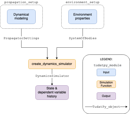
There are two inputs necessary to perform a simulation: a PropagatorSettings instance and a SystemOfBodies instance.
The propagation setup defines the differential equations to be solved and the method to solve them, while the environment setup defines the physical modeling of the environment and system properties, including those of both natural and artificial objects.
See also
For more information on how to setup your environment and propagation, see the user guide on Environment Setup and Propagation Setup.
A core principle of Tudat(Py) is the use of settings objects to define physical models.
A user typically does not create model instances directly, but instead creates (or modifies) a settings object, which is then translated to a model.
Knowing that, we can now start setting up our simulation.
We will first import all necessary modules, including some standard Python modules, like numpy and matplotlib.
# Load standard modules
import numpy as np
from matplotlib import pyplot as plt

# Load tudatpy modules
from tudatpy.interface import spice
from tudatpy import dynamics
from tudatpy.dynamics import environment_setup, propagation_setup
from tudatpy.astro import element_conversion
from tudatpy import constants
from tudatpy.util import result2array
from tudatpy.astro.time_representation import DateTime
See also
For more information about the submodules of Tudat(Py), take a look at the API documentation.
Setting up the environment#
As mentioned before, in Tudat(Py) the physical environment is defined using a SystemOfBodies object.
This object contains all the bodies in the simulation along with their physical properties of these bodies.
In this case, we will define only a central body (Earth) and a satellite.
Tudat(Py) relies heavily on the SPICE toolkit [Acton1996] to retrieve ephemeris data and other planetary information for a number of default bodies. Using the following command
we load a number of default SPICE kernels into TudatPy.
Tip
For a complete list and the order of the default SPICE kernels loaded by TudatPy, see the API documentation on load_standard_kernels().
Define natural bodies#
With the standard kernels loaded, we can define our central body, the Earth.
In this example, the get_default_body_settings() function is used to create the Earth using a number of default settings, which are distributed with Tudat(Py).
# Create default body settings for "Earth"
bodies_to_create = ["Earth"]

# Create default body settings for bodies_to_create, with "Earth"/"J2000" as the global frame origin and orientation
global_frame_origin = "Earth"
global_frame_orientation = "J2000"
body_settings = environment_setup.get_default_body_settings(
   bodies_to_create, global_frame_origin, global_frame_orientation)
See also
For more information on these default models (for ephemeris, rotation, shape, atmosphere, etc.), have a look at Default environment models.
Define artificial bodies#
Because our satellite is an artificial body, it is not known to TudatPy by default.
If we were to add it to bodies_to_create in the previous code block retrieving default settings, TudatPy would throw an error, as our satellite is not a default body.
Instead, we need to create a set of empty body settings for our satellite, using the following code:
# Create empty body settings for the satellite
body_settings.add_empty_settings("Delfi-C3")
Hint
As we are propagating a satellite in a Keplerian orbit, we do not need to define any additional properties for the satellite. For more information on how to define the mass, aerodynamic coefficients or radiation pressure properties of an artificial body, have a look at how to create body settings with additional properties.
Create the system of bodies#
These body settings are then used to create the system of bodies, using the function create_system_of_bodies().
# Create system of bodies
bodies = environment_setup.create_system_of_bodies(body_settings)
We have now defined our environment in the SystemOfBodies instance bodies and are ready to move on to setting up the propagation.
Setting up the propagation#
As mentioned before, the propagation setup defines the differential equations to be solved and the method to solve them. We will first define what to propagate, and then how to propagate it. In this case, we would like to propagate our satellite with respect to the Earth:
# Define bodies that are propagated
bodies_to_propagate = ["Delfi-C3"]

# Define central bodies of propagation
central_bodies = ["Earth"]
Define the acceleration models#
We then define the accelerations acting in our simulation.
This is done by creating a dictionary (acceleration_settings), where the keys are the bodies that undergo an acceleration (in this case only on our satellite), and the values are the accelerations acting on these bodies.
The accelerations acting on our satellite are again defined as a dictionary (acceleration_settings_delfi_c3), with the keys being the bodies, that exert an acceleration on our satellite, and the values being a list of acceleration(s) that each body exerts.
In this case, we only consider the gravitational point-mass acceleration of the Earth acting on the satellite, thus we get:
# Define accelerations acting on Delfi-C3
acceleration_settings_delfi_c3 = dict(
   Earth=[propagation_setup.acceleration.point_mass_gravity()]
)

acceleration_settings = {"Delfi-C3": acceleration_settings_delfi_c3}
Similar to before, we use the function create_acceleration_models() to create the acceleration models from the settings:
# Create acceleration models
acceleration_models = propagation_setup.create_acceleration_models(
   bodies, acceleration_settings, bodies_to_propagate, central_bodies)
See also
In this case, we only considered the influence of a gravitational point-mass attraction. To setup a more complex simulation, have a look at Acceleration Model Setup. To see the full list of available acceleration models, see Available Acceleration Models or the API documentation on accelerations.
Define the initial state#
We would like to simulate our satellite in an elliptical orbit around the Earth.
For the numerical propagation of the translational motion, we need to define the initial state of our satellite in Cartesian elements.
Conveniently, TudatPy has an element_conversion module, which provides a function to convert Keplerian elements to Cartesian elements, keplerian_to_cartesian_elementwise().
In order to convert from Keplerian to Cartesian elements, we also need to know the gravitational parameter of the Earth, which we can simply extract from the environment we created previously:
# Set initial conditions for the satellite that will be
# propagated in this simulation. The initial conditions are given in
# Keplerian elements and later on converted to Cartesian elements
earth_gravitational_parameter = bodies.get("Earth").gravitational_parameter

initial_state = element_conversion.keplerian_to_cartesian_elementwise(
   gravitational_parameter = earth_gravitational_parameter,
   semi_major_axis = 6.99276221e+06, # meters
   eccentricity = 4.03294322e-03, # unitless
   inclination = 1.71065169e+00, # radians
   argument_of_periapsis = 1.31226971e+00, # radians
   longitude_of_ascending_node = 3.82958313e-01, # radians
   true_anomaly = 3.07018490e+00, # radians
)
Hint
In Tudat(Py), all quantities are defined in SI units, with all angular measures defined in radian. All epochs are defined as seconds since J2000 in the TDB scale.
This only leaves the epoch of the initial state to be defined.
We will use Tudat’s own DateTime class to define the epoch of the initial state.
See also
For conversions from other time scales and formats, see Times and dates.
Define the integrator and propagator#
With the acceleration models and initial state defined, we can now define how to propagate the state, i.e. how the differential equations are solved. We will use a simple Runge-Kutta 4 integrator, with a fixed step size of 10 seconds. For the propagator, a Cowell propagator is used, which uses Cartesian elements as the propagated states. Lastly, we define the termination conditions for the propagation, which in this case is a fixed end epoch.
# Create numerical integrator settings
integrator_settings = propagation_setup.integrator.runge_kutta_fixed_step(
   time_step=10.0, coefficient_set=propagation_setup.integrator.rk_4
)

propagator_type = propagation_setup.propagator.cowell

# Create termination settings
termination_settings = propagation_setup.propagator.time_termination(simulation_end_epoch)
Note
Depending on your performance and accuracy requirements, you might want to consider other propagator and integrator combinations. Tudat(Py) offers a variety of other integrators, such as higher-order multi-stage and extrapolation integrators, as well as different propagators, such as the Encke, Keplerian, Modified-Equinoctial, and Unified State Model propagators. For more information, have a look at Integration Setup and the API documentation on propagators.
We are not only interested in the final state of our satellite, but also the evolution of its ground track over time. To retrieve this information, Tudat(Py) uses so-called dependent variables, which store information about the conditions of the system during each step of the integration, in addition to the propagated state itself. We create a list of dependent variables to save, in this case the longitude and latitude of our satellite with respect to the Earth:
# Define list of dependent variables to save
dependent_variables_to_save = [
   propagation_setup.dependent_variable.latitude("Delfi-C3", "Earth"),
   propagation_setup.dependent_variable.longitude("Delfi-C3", "Earth"),
]
See also
For a list of available dependent variables, have a look at the API documentation on dependent variables.
Create the propagator settings#
Putting all together, we can finally create the propagator settings:
# Create propagation settings
propagator_settings = propagation_setup.propagator.translational(
   central_bodies,
   acceleration_models,
   bodies_to_propagate,
   initial_state,
   simulation_start_epoch,
   integrator_settings,
   termination_settings,
   propagator=propagator_type,
   output_variables=dependent_variables_to_save
)
Perform the propagation#
Now that we have defined our PropagatorSettings instance (the propagator_settings object) and a SystemOfBodies instance (the bodies object), we can finally perform the propagation.
As introduced earlier in Setting up the simulation, the propagation is performed using the create_dynamics_simulator() function.
Typically, calling this function performs the propagation (unless the optional input argument simulate_dynamics_on_creation is set to False)
# Create simulation object and propagate the dynamics
dynamics_simulator = dynamics.simulator.create_dynamics_simulator(
   bodies, propagator_settings
)
Post-processing the results#
The create_dynamics_simulator() function returns an instance of a SingleArcSimulator, which has the attribute propagation_results of type SingleArcSimulationResults.
The propagation_results object contains, among other information, the state_history and dependent_variable_history.
The former stores the state of the system at each step of the integration, while the latter holds the dependent variables.
Hint
Both the state_history and dependent_variable_history are stored in the form of dictionaries, which contain the epochs of each single integration step as keys and the corresponding quantities as values.
To post-process the results, we will first convert the state and dependent variable history dictionaries to a NumPy array, which can be easily manipulated and plotted.
TudatPy offers a utility function, result2array(), to convert the dictionaries to NumPy arrays:
# Extract the resulting state history and convert it to an ndarray
states = dynamics_simulator.propagation_results.state_history
states_array = result2array(states)

# Extract the resulting dependent variable history and convert it to an ndarray
dependent_variables = dynamics_simulator.propagation_results.dependent_variable_history
dependent_variables_array = result2array(dependent_variables)
Print the initial and final states#
print(
   f"""
Single Earth-Orbiting Satellite Example.
The initial position vector of Delfi-C3 is [km]: \n
{states[simulation_start_epoch][:3] / 1E3}
The initial velocity vector of Delfi-C3 is [km/s]: \n
{states[simulation_start_epoch][3:] / 1E3} \n
After {simulation_end_epoch - simulation_start_epoch} seconds the position vector of Delfi-C3 is [km]: \n
{states[simulation_end_epoch][:3] / 1E3}
And the velocity vector of Delfi-C3 is [km/s]: \n
{states[simulation_end_epoch][3:] / 1E3}
"""
)
The expected output is:
Single Earth-Orbiting Satellite Example.
The initial position vector of Delfi-C3 is [km]:
[-2455.85398258     8.89844018 -6577.35622264]
The initial velocity vector of Delfi-C3 is [km/s]:
[ 6.47108513  2.97329684 -2.41447086]

After 86400.0 seconds the position vector of Delfi-C3 is [km]:
[-6341.67824913 -2259.72932298 -1943.73703997]
And the velocity vector of Delfi-C3 is [km/s]:
[ 1.55732231  1.71542799 -7.16926862]
Visualize the trajectory#
Finally, let’s visualize the trajectory of our satellite in 3D around Earth.
For this, we use the states_array we previously created with the result2array() function.
The array contains the epochs as the first column, followed by the Cartesian states (position and velocity, with respect to Earth) in SI units.
# Define a 3D figure using pyplot
fig = plt.figure(figsize=(6,6), dpi=125)
ax = fig.add_subplot(111, projection='3d')
ax.set_title(f'Delfi-C3 trajectory around Earth')

# Plot the positional state history
ax.plot(states_array[:, 1], states_array[:, 2], states_array[:, 3], label=bodies_to_propagate[0], linestyle='-.')
ax.scatter(0.0, 0.0, 0.0, label="Earth", marker='o', color='blue')

# Add the legend and labels, then show the plot
ax.legend()
ax.set_xlabel('x [m]')
ax.set_ylabel('y [m]')
ax.set_zlabel('z [m]')
plt.show()
This should give you a 3D plot similar to the following:

Similarly, we will use the dependent variables array to plot the ground track of our satellite on Earth. As with the state history, the dependent variable history is stored in the form of a NumPy array, with the epochs as the first column and the dependent variables as the following columns. We use the epochs to extract a subset of 3 hours of data, for which we plot the ground track:
fig, ax = plt.subplots(tight_layout=True)

latitude = dependent_variables_array[:, 1]
longitude = dependent_variables_array[:, 2]

# Extract 3 hours data subset
relative_time_hours = (dependent_variables_array[:, 0] - simulation_start_epoch) / 3600
hours_to_extract = 3
propagation_span_hours = (simulation_end_epoch - simulation_start_epoch) / 3600

subset = int(len(relative_time_hours) / propagation_span_hours * hours_to_extract)

latitude = np.rad2deg(latitude[:subset])
longitude = np.rad2deg(longitude[:subset])

# Plot ground track
ax.set_title("3 hour ground track of Delfi-C3")
ax.scatter(longitude, latitude, s=1)
ax.scatter(longitude[0], latitude[0], label="Start", color="green", marker="o")
ax.scatter(longitude[-1], latitude[-1], label="End", color="red", marker="x")

# Configure plot
ax.set_xlabel("Longitude [deg]")
ax.set_ylabel("Latitude [deg]")
ax.set_xlim([-180, 180])
ax.set_ylim([-90, 90])
ax.set_xticks(np.arange(-180, 181, step=45))
ax.set_yticks(np.arange(-90, 91, step=45))
ax.legend()
ax.grid(True)
plt.show()
This should give you a plot similar to the following:

Congratulations! You have now successfully propagated a satellite in a Keplerian orbit around the Earth using Tudat(Py) and used the results to visualize its trajectory.
See also
For more information on how to set up more complex simulations, have a look at the examples. They include examples on more complex propagations, such as including additional perturbation models or the effect of a thruster.
If you are interested in using TudatPy for state estimation, have a look at the example of using TudatPy for parameter estimation of Delfi-C3.
Last but not least, if you would like to find the optimal Earth-Mars launch window, you might be interested in using TudatPy to create Porkchop plots.