

Note
Generated by nbsphinx from a Jupyter notebook. All the examples as Jupyter notebooks are available in the tudatpy-examples repo.
Walker constellation propagation#
Objectives#
This example shows how to set up and propagate a satellite constellation using Tudat’s multi-body propagation facilities. It demonstrates a multi-shell architecture in the style of Starlink: two Walker constellations at different altitudes and inclinations, propagated jointly under Earth’s spherical-harmonic gravity field and third-body perturbations from the Sun and Moon.
The two shells are:
Shell |
Walker T/P/F |
Altitude |
Inclination |
Purpose |
|---|---|---|---|---|
A |
24 / 3 / 1 |
550 km |
53.0° |
Mid-latitude coverage |
B |
12 / 3 / 1 |
560 km |
97.6° |
Sun-synchronous polar coverage |
Total: 36 satellites propagated over 24 hours.
What this example shows:
Programmatic generation of Walker-constellation Keplerian elements
Multi-shell concatenation (each shell built with the same generator, then combined)
Multi-body environment + propagation setup at scale
3D visualization of orbits, ground tracks, and in-plane spacing
The osculating-vs-mean-element drift that motivates stationkeeping in real constellations
Import statements#
First, let’s import the needed python and tudat libraries, and let’s load the standard SPICE kernels.
[1]:
# Standard modules
import numpy as np
from matplotlib import pyplot as plt
from mpl_toolkits.mplot3d import Axes3D  # noqa: F401  (registers the 3d projection)

# Tudatpy modules
from tudatpy import constants
from tudatpy import dynamics
from tudatpy.astro import element_conversion
from tudatpy.astro.time_representation import DateTime
from tudatpy.interface import spice
from tudatpy.dynamics import (
    environment_setup,
    propagation_setup,
    propagation,
    simulator,
)

# Load NAIF SPICE kernels (Earth, Sun, Moon ephemerides + rotation models)
spice.load_standard_kernels()
Walker constellation parameters#
Two shells defined as plain dictionaries. Each shell is itself a Walker delta constellation T/P/F, where:
Tis the total number of satellites in the shell,Pis the number of orbital planes (soT/Psatellites per plane),F ∈ [0, P-1]is the phasing factor (the relative angular offset between adjacent planes’ satellites at the ascending node).
See the Walker constellation summary on Wikipedia for an accessible derivation. We use Earth’s mean radius from SPICE so the shell altitudes resolve to physically correct semi-major axes.
[2]:
# Earth's mean radius from SPICE (meters)
EARTH_RADIUS = spice.get_average_radius("Earth")

# Shell A: Starlink-like mid-latitude shell
shell_A = {
    "name": "A",
    "T": 24,                    # total satellites in this shell
    "P": 3,                     # number of orbital planes
    "F": 1,                     # phasing factor (0..P-1)
    "altitude_m": 550.0e3,      # altitude above Earth's mean radius
    "sma_m": EARTH_RADIUS + 550.0e3,
    "eccentricity": 0.0,        # circular orbit
    "inclination_deg": 53.0,    # mid-latitude (Starlink Shell 1 nominal)
}

# Shell B: polar / sun-synchronous-like shell
shell_B = {
    "name": "B",
    "T": 12,
    "P": 3,
    "F": 1,
    "altitude_m": 560.0e3,
    "sma_m": EARTH_RADIUS + 560.0e3,
    "eccentricity": 0.0,
    "inclination_deg": 97.6,    # polar coverage; near sun-synchronous at this altitude
}

shells = [shell_A, shell_B]
total_sats = sum(s["T"] for s in shells)
print(f"Total satellites across all shells: {total_sats}")
Total satellites across all shells: 36
Walker constellation generator#
Let’s add a utility function, named generate_walker_kepler_elements, that takes a Walker T/P/F specification and a shared orbital geometry (semi-major axis, eccentricity, inclination), and emits one Keplerian-element set per satellite. The formulas are from Walker (1984) — see the Wikipedia summary for an accessible derivation.
[3]:
def generate_walker_kepler_elements(
    T: int,
    P: int,
    F: int,
    sma_m: float,
    eccentricity: float,
    inclination_rad: float,
) -> list:
    """Generate Keplerian elements for a Walker constellation T/P/F.

    Args:
        T: total number of satellites
        P: number of orbital planes (must divide T evenly)
        F: phasing factor (integer in 0..P-1)
        sma_m: semi-major axis in metres (shared across all satellites in this shell)
        eccentricity: eccentricity (typically 0 for constellations)
        inclination_rad: inclination in radians (shared across all satellites)

    Returns:
        List of length T, each entry an np.ndarray shape (6,):
        [sma_m, eccentricity, inclination_rad, argument_of_periapsis_rad,
         RAAN_rad, true_anomaly_rad]
        — exactly the order Tudat's `element_conversion.keplerian_to_cartesian_elementwise` expects.
        Order in the list: all sats of plane 0 first (in true-anomaly order), then plane 1, then plane 2, ...

    See reference doc §2 for the math (RAAN per plane, true anomaly per sat-in-plane, phasing offset).
    """
    assert T % P == 0, "T must devide evenly"
    sats_per_plane = T // P
    result = []
    for k in range(P):
        raan_k = 2 * np.pi * k / P
        for j in range(sats_per_plane):
            true_anomaly_k = (2 * np.pi / sats_per_plane) * j + (2 * np.pi * F / T) * k
            true_anomaly_k %= 2 * np.pi
            kep = np.array([
                sma_m,
                eccentricity,
                inclination_rad,
                0.0,
                raan_k,
                true_anomaly_k,
            ])
            result.append(kep)
    return result
Generate Keplerian elements for all satellites#
Apply the generator to each shell and flatten into a single list of (kep_elements, satellite_name) tuples. Names follow the pattern shell_{A,B}_p{plane}_s{sat_in_plane} and are used as body identifiers throughout Tudat.
[4]:
satellites = []  # list of dicts: {"name": str, "shell": str, "plane": int, "sat_in_plane": int, "kep": np.ndarray}

for shell in shells:
    kep_list = generate_walker_kepler_elements(
        T=shell["T"],
        P=shell["P"],
        F=shell["F"],
        sma_m=shell["sma_m"],
        eccentricity=shell["eccentricity"],
        inclination_rad=np.deg2rad(shell["inclination_deg"]),
    )
    sats_per_plane = shell["T"] // shell["P"]
    for idx, kep in enumerate(kep_list):
        plane = idx // sats_per_plane
        sat_in_plane = idx % sats_per_plane
        name = f"shell_{shell['name']}_p{plane}_s{sat_in_plane}"
        satellites.append({
            "name": name,
            "shell": shell["name"],
            "plane": plane,
            "sat_in_plane": sat_in_plane,
            "kep": kep,
        })

print(f"Generated Keplerian elements for {len(satellites)} satellites.")
print(f"First sat: {satellites[0]['name']} → kep = {satellites[0]['kep']}")
Generated Keplerian elements for 36 satellites.
First sat: shell_A_p0_s0 → kep = [6.92100837e+06 0.00000000e+00 9.25024504e-01 0.00000000e+00
 0.00000000e+00 0.00000000e+00]
Create environment and bodies#
We will soon propagate the satellites we created under the gravitational influence of Sun, Earth and Moon. Let’s then create the environment and bodies accordingly: Sun + Earth + Moon from SPICE defaults, plus one empty body per satellite. The empty-body pattern is the standard way to add custom spacecraft — mass and any other properties are set per-satellite after creation. For background see the Tudat user guide on environment setup.
[5]:
# Celestial bodies to load from SPICE defaults
bodies_to_create = ["Sun", "Earth", "Moon"]

global_frame_origin = "Earth"
global_frame_orientation = "J2000"

body_settings = environment_setup.get_default_body_settings(
    bodies_to_create,
    global_frame_origin,
    global_frame_orientation,
)

# Add an empty body for each satellite
SATELLITE_MASS_KG = 260.0  # Starlink v1.5 nominal mass; constant across constellation
for sat in satellites:
    body_settings.add_empty_settings(sat["name"])
    body_settings.get(sat["name"]).constant_mass = SATELLITE_MASS_KG

# Materialize the system
bodies = environment_setup.create_system_of_bodies(body_settings)
print(f"Created {len(bodies_to_create)} celestial bodies + {len(satellites)} satellites.")
Created 3 celestial bodies + 36 satellites.
Acceleration settings#
For LEO at ~550 km, the physically important forces are:
Earth gravity — main term. We use a spherical-harmonic expansion to degree/order 8 (
spherical_harmonic_gravity(8, 8)), which captures J2 (Earth’s oblateness, dominant non-central term) plus higher-order zonal and tesseral terms.Sun and Moon point-mass gravity — third-body perturbations, small but non-trivial over a day.
To keep things simple, atmospheric drag is not included in this example. The same acceleration set applies to every satellite (no per-satellite differentiation in this scope). See the tudatpy acceleration API for the full menu of acceleration settings.
[6]:
# Acceleration set applied to every satellite
accelerations_per_satellite = dict(
    Sun=[propagation_setup.acceleration.point_mass_gravity()],
    Earth=[propagation_setup.acceleration.spherical_harmonic_gravity(8, 8)],
    Moon=[propagation_setup.acceleration.point_mass_gravity()],
)

# Map each satellite name → acceleration spec
acceleration_settings = {sat["name"]: accelerations_per_satellite for sat in satellites}

# All satellites orbit Earth
bodies_to_propagate = [sat["name"] for sat in satellites]
central_bodies = ["Earth"] * len(satellites)

acceleration_models = propagation_setup.create_acceleration_models(
    bodies,
    acceleration_settings,
    bodies_to_propagate,
    central_bodies,
)
Initial Cartesian states#
Tudat propagates in Cartesian inertial coordinates (J2000), so the Keplerian sets must be converted. The result is a single flat vector of length 6 * N where the first 6 entries are sat 0, the next 6 are sat 1, and so on — same order as bodies_to_propagate.
Cartesian conversion uses tudatpy’s `element_conversion.keplerian_to_cartesian_elementwise <https://py.api.tudat.space/en/latest/element_conversion.html#tudatpy.astro.element_conversion.keplerian_to_cartesian_elementwise>`__.
[7]:
# Convert each Keplerian set to Cartesian, then concatenate into a single flat
# state vector of shape (6 * N_total_sats,) in the same order as `satellites`.

earth_mu = bodies.get("Earth").gravitational_parameter

initial_states_list = []
for sat in satellites:
    cartesian = element_conversion.keplerian_to_cartesian_elementwise(
        gravitational_parameter=earth_mu,
        semi_major_axis=sat["kep"][0],
        eccentricity=sat["kep"][1],
        inclination=sat["kep"][2],
        argument_of_periapsis=sat["kep"][3],
        longitude_of_ascending_node=sat["kep"][4],
        true_anomaly=sat["kep"][5],
    )
    sat["cartesian_initial"] = cartesian
    initial_states_list.append(cartesian)

initial_states = np.concatenate(initial_states_list)
Dependent variables to save#
We save the full Keplerian state for every satellite at every integration step. This is needed for the in-plane spacing analysis (post-processing §3) and is also useful for verifying the constellation is behaving as expected.
[8]:
dependent_variables_to_save = [
    propagation_setup.dependent_variable.keplerian_state(sat["name"], "Earth")
    for sat in satellites
]
Termination and integrator settings#
Propagate over 24 hours (a full diurnal cycle for ground-track visualization). Use a variable-step Runge-Kutta-Fehlberg 7(8) integrator — a sensible default for LEO propagation.
[9]:
# Simulation epochs
simulation_start_epoch = DateTime(2000, 1, 1).to_epoch()
simulation_end_epoch = simulation_start_epoch + constants.JULIAN_DAY  # 24 hours

# Time-based termination
termination_settings = propagation_setup.propagator.time_termination(simulation_end_epoch)

# Variable-step RKF 7(8)
integrator_settings = propagation_setup.integrator.runge_kutta_variable_step_size(
    initial_time_step=10.0,
    coefficient_set=propagation_setup.integrator.CoefficientSets.rkf_78,
    minimum_step_size=1.0,
    maximum_step_size=100.0,
    relative_error_tolerance=1.0e-10,
    absolute_error_tolerance=1.0e-10,
)

# Translational propagation settings
propagator_settings = propagation_setup.propagator.translational(
    central_bodies,
    acceleration_models,
    bodies_to_propagate,
    initial_states,
    simulation_start_epoch,
    integrator_settings,
    termination_settings,
    output_variables=dependent_variables_to_save,
)
Run the simulation#
This is the actual numerical propagation. With 36 satellites over 24 hours under spherical-harmonic gravity, expect this to take several seconds — the spherical-harmonic expansion is the heaviest term.
[10]:
dynamics_simulator = simulator.create_dynamics_simulator(bodies, propagator_settings)

state_history = dynamics_simulator.propagation_results.state_history
dependent_variable_history = dynamics_simulator.propagation_results.dependent_variable_history

epochs = np.array(list(state_history.keys()))
state_array = np.array(list(state_history.values()))         # shape (n_steps, 6 * N_sats)
dep_var_array = np.array(list(dependent_variable_history.values()))  # shape (n_steps, 6 * N_sats)

print(f"Propagated {len(epochs)} integration steps over "
      f"{(epochs[-1] - epochs[0]) / 3600:.1f} hours.")
print(f"State array shape: {state_array.shape}")
Propagated 908 integration steps over 24.0 hours.
State array shape: (908, 216)
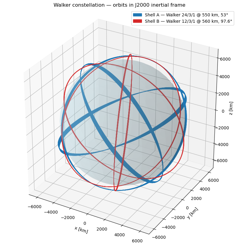
Post-processing 1 — 3D orbital geometry#
Render all satellite orbits in inertial space, colored by shell (Shell A blue, Shell B red), with Earth as a reference sphere.
These positions are in J2000 inertial — see the Tudat user guide on coordinate frames for the reference frame definitions.
[11]:
# 3D plot of all satellite orbits, colored by shell.
import matplotlib.patches as mpatches

fig = plt.figure(figsize=(10, 10))
ax = fig.add_subplot(111, projection="3d")

# Earth reference sphere
earth_r_km = EARTH_RADIUS / 1000.0
u = np.linspace(0, 2 * np.pi, 60)
v = np.linspace(0, np.pi, 30)
x_earth = earth_r_km * np.outer(np.cos(u), np.sin(v))
y_earth = earth_r_km * np.outer(np.sin(u), np.sin(v))
z_earth = earth_r_km * np.outer(np.ones_like(u), np.cos(v))
ax.plot_surface(x_earth, y_earth, z_earth, alpha=0.2, color="lightblue", linewidth=0)

# Per-satellite orbit, colored by shell
shell_color = {"A": "tab:blue", "B": "tab:red"}
for i, sat in enumerate(satellites):
    x = state_array[:, 6 * i + 0] / 1000.0
    y = state_array[:, 6 * i + 1] / 1000.0
    z = state_array[:, 6 * i + 2] / 1000.0
    ax.plot(x, y, z, color=shell_color[sat["shell"]], alpha=0.5, linewidth=0.8)

# Legend with one entry per shell
legend_handles = [
    mpatches.Patch(color=shell_color["A"], label="Shell A — Walker 24/3/1 @ 550 km, 53°"),
    mpatches.Patch(color=shell_color["B"], label="Shell B — Walker 12/3/1 @ 560 km, 97.6°"),
]
ax.legend(handles=legend_handles, loc="upper right")

ax.set_xlabel("x [km]")
ax.set_ylabel("y [km]")
ax.set_zlabel("z [km]")
ax.set_title("Walker constellation — orbits in J2000 inertial frame")

# Enforce equal axis limits so the Earth actually renders as a sphere — matplotlib
# auto-scales each 3D axis independently otherwise, which squashes the globe.
all_coords = np.concatenate([
    state_array[:, 6 * i + j] / 1000.0
    for i in range(len(satellites)) for j in range(3)
])
lim = max(np.max(np.abs(all_coords)), earth_r_km * 1.1)
ax.set_xlim(-lim, lim)
ax.set_ylim(-lim, lim)
ax.set_zlim(-lim, lim)
ax.set_box_aspect([1, 1, 1])
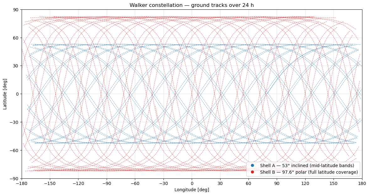
Post-processing 2 — ground tracks#
Project sub-satellite points (the point on Earth’s surface directly below each satellite) onto a 2D lat/lon map. This visualization makes the multi-shell architecture obvious: Shell A’s 53°-inclined orbits trace mid-latitude bands, while Shell B’s 97.6° polar orbits cover all latitudes including the poles.
Important: ground tracks need positions in the Earth-fixed (ECEF) frame, not J2000 inertial — the Earth is rotating beneath the orbit. The rotation comes from Tudat’s Earth rotation model via bodies.get("Earth").rotation_model.inertial_to_body_fixed_rotation(epoch).
[12]:
# Ground tracks: compute sub-satellite latitude/longitude via J2000 → ECEF rotation
import matplotlib.lines as mlines

earth_rotation_model = bodies.get("Earth").rotation_model

n_steps = len(epochs)
n_sats = len(satellites)
lats = np.zeros((n_steps, n_sats))
lons = np.zeros((n_steps, n_sats))

for t_idx, epoch in enumerate(epochs):
    R_j2000_to_ecef = earth_rotation_model.inertial_to_body_fixed_rotation(float(epoch))
    for i in range(n_sats):
        r_j2000 = state_array[t_idx, 6 * i : 6 * i + 3]
        r_ecef = R_j2000_to_ecef @ r_j2000
        r_norm = np.linalg.norm(r_ecef)
        lats[t_idx, i] = np.rad2deg(np.arcsin(r_ecef[2] / r_norm))
        lons[t_idx, i] = np.rad2deg(np.arctan2(r_ecef[1], r_ecef[0]))

# Plot two satellites per shell as dashed lines — keeps the figure readable
# while preserving each shell's characteristic ground-track shape. Indices
# 0, 1 are in Shell A (24 sats); 34, 35 are in Shell B (last two).
shell_color = {"A": "tab:blue", "B": "tab:red"}

def _mask_wrap(arr):
    out = arr.astype(float).copy()
    jumps = np.abs(np.diff(out, axis=0)) > 180.0
    out[1:][jumps] = np.nan
    return out

lons_plot = _mask_wrap(lons)

fig, ax = plt.subplots(figsize=(14, 7))
for i in (0, 1, 34, 35):
    ax.plot(lons_plot[:, i], lats[:, i],
            c=shell_color[satellites[i]["shell"]],
            linestyle="--", alpha=0.6, linewidth=0.8)

ax.set_xlim(-180, 180)
ax.set_ylim(-90, 90)
ax.set_xticks(np.arange(-180, 181, 30))
ax.set_yticks(np.arange(-90, 91, 30))
ax.set_xlabel("Longitude [deg]")
ax.set_ylabel("Latitude [deg]")
ax.set_title("Walker constellation — ground tracks over 24 h")
ax.grid(True, alpha=0.3)

# Proxy legend (scatter does not auto-legend nicely)
legend_handles = [
    mlines.Line2D([], [], color=shell_color["A"], marker="o", linestyle="None",
                  label="Shell A — 53° inclined (mid-latitude bands)"),
    mlines.Line2D([], [], color=shell_color["B"], marker="o", linestyle="None",
                  label="Shell B — 97.6° polar (full latitude coverage)"),
]
ax.legend(handles=legend_handles, loc="lower right")
[12]:
<matplotlib.legend.Legend at 0x1345be4d0>
Post-processing 3 — in-plane spacing analysis and it’s drift#
Plot the angular separation between adjacent satellites in Shell A, plane 0. Initially these 8 satellites are spaced exactly 45° apart (= 360° / (T/P) = 360° / 8). We measure spacing directly from position vectors via arccos(r̂₁ · r̂₂) — this is singularity-free for circular orbits where the Keplerian true anomaly is degenerate.
What we observe: the spacing is not staying at 45°. It drifts by ~7° over 24 hours, with an alternating pattern by satellite-pair index (adjacent pairs split into two bundles, one drifting up to ~52°, the other down to ~38°).
Why#
We initialised all 8 satellites with identical osculating Keplerian elements (same a, e, i, Ω, ω) but different ν. Tudat then faithfully integrates Newton + J2 in Cartesian coordinates.
And since the osculating elements differ from the mean (Brouwer-Lyddane) elements by short-period oscillations, the amplitude of which depends on the instantaneous phase of the satellite, even though all eight satellites have identical osculating semi-major axes of a = 6921 km, their mean semi-major axes differ slightly by an amount dependent on phase:
Different mean a ⇒ different mean motion ⇒ slow secular drift in along-track position between satellites. The order-of-magnitude derivation:
The short-period \(J_2\) contribution to the semi-major axis scales as \(\delta a / a \sim J_2 (R_\oplus / a)^2\). For LEO at \(a \approx R_\oplus + 550\,\text{km}\) with \(J_2 \approx 1.083 \times 10^{-3}\), this gives \(\delta a / a \sim 10^{-3}\) (the leading factor swallows the \((R_\oplus/a)^2 \approx 0.85\)).
From Kepler’s third law \(n \propto a^{-3/2}\), hence \(\delta n / n = -\tfrac{3}{2}\,\delta a / a \sim 10^{-3}\).
Over 15 orbits (24 h at a ~95-min period), the cumulative along-track phase difference between two sats whose mean \(a\) differ by this amount is \(\sim 15 \times 10^{-3} \times 360° \approx 5\text{--}7°\) — which is consistent with what we see in the plot.
The alternating two-bundle pattern comes from the 2-per-orbit phase dependence of \(\delta a_{J_2}(\nu)\): satellites 180° apart in true anomaly see identical short-period offsets, producing the 4-fold pair-index symmetry visible in the plot.
This is the dominant cause: replacing the full spherical_harmonic_gravity(8, 8) + Sun + Moon set-up with only J2 (no tesserals, no 3rd-body) gives essentially the same drift (within 0.2°). Higher-order zonals, tesserals, and 3rd-body perturbations contribute small additional effects on top of the J2-driven mean-element separation.
How to fix#
To preserve Walker geometry exactly in simulation, you would invert the Brouwer-Lyddane mean-to-osculating transformation: choose osculating initial conditions per satellite such that the mean elements are uniform across the constellation. This is left out of scope of this example.
Further reading:
Curtis, Orbital Mechanics for Engineering Students (4th ed.), Ch. 10 — Orbital perturbations
Vallado, Fundamentals of Astrodynamics and Applications (4th ed.), §9.3 — Special perturbations
Brouwer (1959), “Solution of the problem of artificial satellite theory without drag”, Astron. J. 64, 378
[13]:
# In-plane angular spacing for Shell A, plane 0 — verifies Walker geometry is preserved during propagation
target_shell, target_plane = "A", 0

target_indices = [
    i for i, s in enumerate(satellites)
    if s["shell"] == target_shell and s["plane"] == target_plane
]
n_target = len(target_indices)

shell_config = next(s for s in shells if s["name"] == target_shell)
expected = shell_config["T"] // shell_config["P"]
assert n_target == expected, f"expected {expected} sats, got {n_target}"
ideal_spacing_deg = 360.0 / n_target
print(f"Shell {target_shell} plane {target_plane}: {n_target} sats, ideal spacing {ideal_spacing_deg:.1f}°")

# Extract position vectors for the target sats: shape (n_steps, n_target, 3)
positions = np.zeros((len(epochs), n_target, 3))
for j, sat_idx in enumerate(target_indices):
    positions[:, j, :] = state_array[:, 6 * sat_idx : 6 * sat_idx + 3]

# Pairwise adjacent angular separations via arccos(r̂₁ · r̂₂)
# (singularity-free; works whether the underlying tЧасть пар спутников (верхний пучок) непрерывно увеличивает дистанцию между собой (угол растет к 52°), а другая часть (нижний пучок) — догоняет друг друга (угол падает к 38°).rue anomaly is well-defined or not)
hours = (epochs - epochs[0]) / 3600.0
pairs = [(j, (j + 1) % n_target) for j in range(n_target)]

fig, ax = plt.subplots(figsize=(10, 5))
for j_start, j_end in pairs:
    r1 = positions[:, j_start, :]
    r2 = positions[:, j_end, :]
    cos_theta = np.einsum("ij,ij->i", r1, r2) / (
        np.linalg.norm(r1, axis=1) * np.linalg.norm(r2, axis=1)
    )
    cos_theta = np.clip(cos_theta, -1.0, 1.0)  # protect arccos from numerical >1 or <-1
    angle_deg = np.rad2deg(np.arccos(cos_theta))
    ax.plot(hours, angle_deg, label=f"sat {j_end} − sat {j_start}", linewidth=0.8)

ax.axhline(ideal_spacing_deg, color="gray", linestyle="--", alpha=0.7,
           label=f"ideal ({ideal_spacing_deg:.1f}°)")
ax.set_xlabel("Time [h]")
ax.set_ylabel("In-plane angular separation [deg]")
ax.set_title(f"In-plane spacing — Shell {target_shell}, plane {target_plane} "
             f"({n_target} satellites)")
ax.grid(True, alpha=0.3)
ax.legend(loc="lower right", fontsize=8, ncol=2)
ax.set_xlim(0, hours[-1])

# Diagnostic: print min/max spacing across all pairs, all times
all_spacings = []
for j_start, j_end in pairs:
    r1 = positions[:, j_start, :]
    r2 = positions[:, j_end, :]
    cos_theta = np.clip(
        np.einsum("ij,ij->i", r1, r2) / (np.linalg.norm(r1, axis=1) * np.linalg.norm(r2, axis=1)),
        -1.0, 1.0,
    )
    all_spacings.append(np.rad2deg(np.arccos(cos_theta)))
all_spacings = np.concatenate(all_spacings)
print(f"Spacing range over 24 h: min={all_spacings.min():.3f}°, max={all_spacings.max():.3f}°, "
      f"std={all_spacings.std():.4f}° (ideal {ideal_spacing_deg:.1f}°)")
Shell A plane 0: 8 sats, ideal spacing 45.0°
Spacing range over 24 h: min=37.876°, max=52.179°, std=4.1132° (ideal 45.0°)

Show all figures#
Required to render the figures in jupyter.
[14]:
plt.show()
Where to go from here#
This example deliberately keeps scope tight, so that the focus stays on the constellation-setup pattern itself. There are several natural directions in which to extend it, each substantial enough to make a good follow-up notebook on its own.
The first is drag and atmosphere modelling: at 550 km the atmosphere still has a measurable effect on the orbit, and adding per-satellite aerodynamic coefficients together with an atmosphere model lets us watch the constellation gradually decay — and lets us reason about the stationkeeping budget required to maintain it. Solar radiation pressure sits in the same family: smaller in magnitude, but real, and the per-satellite SRP-coefficient pattern is the same.
A second direction is inter-satellite-link geometry: compute pairwise line-of-sight visibility (optionally accounting for Earth occultation) over time. That is the natural step toward any constellation-tasking or relay study. Close to that is ground-coverage analysis: for a chosen set of ground points, compute satellite visibility windows and aggregate them across shells to quantify the coverage gain of adding a polar shell.
Finally, the J2-driven drift discussed above motivates maneuver planning: periodic stationkeeping burns to compensate the secular along-track separation, or coordinated burns for constellation reconfiguration. Both fit on top of the same Walker generator presented here.